Data Screening Tutorial

This topic is a mini-tutorial that describes how the data screening tools can be applied to an actual data set.  It may be enough to get you started if you want to avoid plowing through the help file from start to finish.  For a more complete description of the pertinent dialogs, and for a more detailed explanation of the displayed numbers, see Geometry Page and Traverse Page.

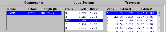
When you compile a project tree branch and observe the Geometry page of the review dialog you may see several "Loop Systems" listed for the network fragment that's highlighted under "Components".  Only multiple-traverse systems are listed in this upper list box.  (A lower 1-item list box is used to select the 1-traverse systems as a group.)  Those systems with the worst statistics, or largest combined UVEs, are listed first.  A "Traverses" list box on the right shows the traverses for the selected system, also arranged with the worst entries at the top.  For example, here is the top part of the Geometry page as it appears after compiling Paxton Cave, a 7-mile long, 327-loop maze:

The game you play while data screening is "float or correct all traverses with conspicuously large F-ratios while reducing each loop system's UVE to as small a value as possible".  In the process you should locate and correct bad measurements within traverses, or single out whole traverses that are so obviously incompatible that they should be permanently floated so they don't distort the map.  What size UVEs to expect will obviously depend on many factors.  (See Variance Assignments.)   My experience has been that a single surveying team employing Suuntos and fiberglass tape can consistently achieve UVEs (both horizontal and vertical) smaller than 1.0.  In a large project involving multiple teams, UVEs less than 2.0 might be a more realistic goal.

The results for Paxton Cave meet these expectations almost perfectly.  The horizontal and vertical UVEs (all systems combined) are a remarkable 1.00 and 1.02, respectively.  We'll use this data set, exactly as it was provided to me by Bob Thrun, to illustrate some powerful data screening techniques.  In the process we'll quickly locate several errors whose obvious fixes would lower the vertical UVE to 0.75.

First, note that we've highlighted the cave's largest loop system, which has 787 total traverses and a vertical UVE (UveV) of 1.02.  We've also selected the system's worst traverse, one that shows "48.7/ 0.88" in the F/UveV column.  The top number (48.7) is the F-ratio, which measures the traverse's "agreement" with all other traverses in the loop system.  A value of zero represents perfect agreement.  A value of one is close to the expected agreement.  In this case, F is much greater than one, which means that the system's vertical consistency will improve significantly if this traverse alone is discarded.  In fact, UveV will drop from 1.02 to 0.88 (the number beneath the slash).  If F had been smaller than one, detaching the traverse would actually worsen consistency; the number beneath the slash would have been larger than 1.02.  Hence the bottom number is what the new UveV will be after the traverse is discarded -- something we can immediately verify by clicking the "FloatV" button.

Before continuing with this example, I should comment about the statistics in general.  Our approach is not to apply formal rules to automatically identify and reject bad measurements.  Although we could determine the probability that an F-ratio will have a value less than X given certain assumptions, a less formal approach based on experience with real data is far more effective in my opinion.  It's not hard to quickly get a feel for the statistics as we locate "outlier" traverses and confirm they are caused by blunders of various kinds.  I suggest that in a sufficiently large and debugged loop system -- say with a loop count of at least 5 -- the F-ratios should be fairly smoothly distributed between 0 and 5, with perhaps a few between 5 and 10.  Anything above 7 is certainly sufficient cause to recheck the field notes.  When a loop system is very large, with hundreds of traverses, the system UVEs could be within tolerance even when some outstanding F-ratios reveal several outliers.  The Paxton Cave example demonstrates this.  It's therefore important to screen all loop systems -- even those with small UVEs.

Graphical Review

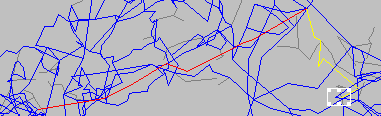
Once we highlight a traverse near the top of the list there are two routes to follow in discovering why its numbers are so bad -- possibly so bad as to be unprintable, in which case you'll see a set of dashes: "--.-".  What I would probably do first is click one (or both) of the "FloatV/FloatH" buttons underneath the list box.  This reprocesses the loop system and refreshes the displayed statistics; the respective components of the traverse are effectively thrown out.  Immediately after this I would click the "Zoom" button to display the dialog's Map page homed in to the floated traverse.  Shown in yellow is the uncorrected raw traverse as it was originally measured.  Shown in red is the traverse as it would now be seen on a printed map.  The red version "floats" to fit the now independently adjusted network.  If we had zoomed without floating first, we would see only a red adjusted version and the network around it would likely be distorted by its effect.  After floating the worst (topmost) traverse in Paxton Cave and then zooming in to its profile, we would see something like this:

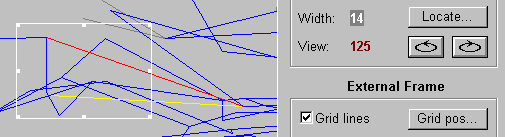
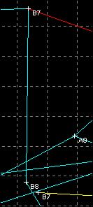
At this point, common problems like misnamed stations, reversed From/To names, and reversed signs on inclinations should be easy to spot.  You may want to click the tool bar button that toggles between attaching one end or the other of the yellow traverse to the corresponding network station.  In this particular case, however, we see that the correct end is already attached.  Obviously a shot was made from the bottom of a 6-foot vertical drop rather than from its top, as the data wrongly implies.  To see a map with station labels we need only click the Display button in the "Displayed or Printed Map" section of the control panel.

Review Best Correction

The other route to follow is the Traverse page of the Review dialog.  (Double clicking on a list box item in the Geometry page is a quick way to select a particular traverse while switching to the Traverse page at the same time.)  This page shows the uncorrected vectors of the selected traverse in their proper sequence, each transformed into spherical coordinate measurements whether or not they were derived from compass and tape data.  These measurements may not reflect their original units, but this is not normally a problem if you realize that the declination, convergence, and instrument corrections have already been applied to obtain true north (or grid-relative) bearings.  There is a check box in the upper right corner of the page that toggles between feet and meters.

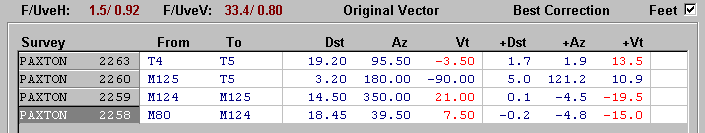
Above is the top portion of the Traverse page as it would appear after selecting the third traverse listed for Paxton Cave's big system.  This traverse originally had the second worst vertical F (28.4).  Now that we've detached the misnamed station, its new vertical F of 33.4 happens to be the worst.  To the right of each raw vector is a set of three corresponding measurement increments, or suggested corrections.  If all three increments for just one vector were to be applied then the traverse would close perfectly with the remaining network (adjusted with that traverse omitted from the data) and both F-ratios would be zero.  The closure vector, the traverse's best correction, can be inferred from the increments, but it's also displayed as east-north-up components at the bottom of the Traverse page (not seen here).  By definition, the best correction is the same whether or not the traverse has been floated; there's no need to float a traverse before examining it on the Traverse page.  However, floating or correcting other traverses first, if they are bad, will often affect these numbers, making them more likely to match an actual error in the data.

As illustrated above, several of the traverse's vectors can have measurements and corresponding increments highlighted in red.  Each of the three measurement types (distance, bearing, and inclination ) has a user specified tolerance level, in this case 3 feet, 5 degrees, and 5 degrees.  (See Options | Compilation | Vector Highlighting... in the Walls menu.)  If exactly one of the increments is out of tolerance, then both it and its corresponding measurement are colored red instead of blue.  Thus attention is drawn immediately to any single measurement that would alone fix the traverse if corrected.

Here we see that three of four traverse vectors meet this criterion.  Of the three inclination corrections that are highlighted, the last one in particular gets our attention: namely -15.0, which when added to the original 7.50 measurement amounts to a sign reversal.  Of course we would examine the notes and sketch if they were available, but without them we strongly suspect that "-7.5" instead of "7.5" should have been recorded for shot M80 to M124.  The other possibilities are less likely but can't be discounted entirely.  For example, the second vector (M125 to T5) fails to meet our criterion for highlighting, but perhaps we should treat this pure vertical shot as a special case.  Simply changing this vertical distance from "3.2" to "8.2" would eliminate the traverse's vertical misclosure while having no effect on horizontal consistency.

We can continue in this fashion.  For example, floating this traverse produces a new set of statistics, the worst vertical F (29.8) now belonging to a 3-vector traverse with a sign reversal even more obvious than the one just diagnosed.  The Traverse page suggests we add -26.6 to the 13.0 inclination measurement in shot A11 to A12.  Likewise, we can focus attention on the system's horizontal statistics, the worst being a horizontal F of 22.0 for the second traverse listed.   Here a -6.8 foot correction in distance is suggested for shot HC37 to HC18.  Perhaps "21.1" was mistaken for "27.1".  The next worst horizontal F happens to be for a pair of chained traverses .  Such traverses necessarily have identical statistics and can be treated as if they formed a single traverse.  Within them several suspicious measurements are highlighted, and it would take just a few minutes to check them against the field notes if they were available.  Overall, the horizontal consistency is remarkably good.  After floating just five of the 787 traverses, the horizontal UVE is reduced from 0.99 to 0.81 with F-ratios all in the single-digit range.

Finally we come to the most gratifying step in the process.  Once we are in the Traverse page, we can double-click a vector to open an edit window into the appropriate survey file, with the vector's data line highlighted.  We will be doing this often to correct mistakes we've confirmed by examining our notes.  Although it's often possible to winnow out multiple bad traverses interactively by simply floating them in succession as we've done here, it's usually better to correct mistakes as soon as we find them and recompile.  This way the new data can play a role in exposing further inconsistencies.

The Paxton Cave survey data was obviously in very good shape when I received it.  It's also characteristic of a dense horizontal maze.  I'll finish this overview with something closer to what you'll encounter if you use Walls with some existing large project data sets.  Multiple blunders in systems with significant vertical relief can actually be fun to ferret out.

Below is a 500-foot wide plan view of part of Lechuguilla Cave's "South" survey as it was sent to me by Dale Pate in June, 1996.  Highlighted in the Map page's preview map is the topmost listed traverse after thirty of 643 traverses were successively floated -- a mechanical process in which simply the worst remaining traverse was floated at each step.  This brought the horizontal UVE of a 258-loop system down to 6.7 from an initial high of 224.4, with the horizontal F finally ranging from 0 to 10.

Our hope is that this initial screening phase leaves us with enough good data (613 traverses) to help us in the next phase: determining why each floated traverse is so grossly inconsistent.  As it happens, many of the traverses are bad simply because their endpoints are misnamed, and we can make several fixes without even referring to the original notes.  For example, the free end of the traverse highlighted above, which is named FNHA3 in the data, comes to within 7 feet horizontally and 2 feet vertically of FNHC3.  (If we had omitted the first phase and floated this traverse alone, it would have come to within 14 ft and 5 ft, respectively.)  No other station in the vicinity is this close in either dimension nor has a name this similar to FNHA3.  The real FNHA3 is about 400 ft horizontally and 160 ft vertically away from FNHC3.

In projects like Lechuguilla Cave, one can easily imagine how useless unadjusted plots of the entire data set would be in trying to specifically identify such problems.  You'll notice that Walls doesn't even offer the option of producing a plot in which the selection of detached traverses is completely arbitrary.  (You can instead highlight all floated traverses on the map.)  Likewise, the common approach of examining residuals (also known as "error ratios"), which are based on how much each traverse is actually corrected by a single all-encompassing adjustment, would be of very little help.

Additional Notes On the Statistics

If you use this program extensively you will occasionally see a large vertical component F-ratio, even though the containing loop system's vertical UVE may in fact be strikingly small.  You'll recognize this as a loop system (usually a small one) where almost all of the vertical angle measurements are exactly zero, resulting in near perfect vertical closure.  In this case, even though a traverse's vertical error may be acceptable (but nonzero), its corresponding F-ratio could be quite large.  You might see "--.-/0.01" in the F/UveV column of the Geometry page.  Obviously, statistics inflated by such circumstances are no cause for concern.

This illustrates an important property of F-ratios compared to UVEs.  Unlike a loop system's UVE, which is sensitive to the magnitude of assigned variances, an F-ratio does not depend on any prior notion of what constitutes a "small error" when evaluating a traverse's misclosure.  The basis for comparison implicit in an F-ratio is just the internal consistency achieved by other traverses in the particular loop system being examined.  (An isolated loop is a special case, where we have decided to use all other isolated loops as the basis for comparison.)

Given the likelihood of multiple blunders in large loop systems, the F-ratios are more useful for the relative ranking of traverses within a single system than for comparing traverses in different systems.  In a system where many of the traverse measurements are bad, the F-ratios could all be small in magnitude (say, less than 7), with the UVEs after detachment all in the double-digit range.  This situation is easily created by accidentally mixing different surveys with duplicated station names, or by combining the work of teams using uncalibrated compasses.  It is primarily for this reason that Walls displays for each traverse both the F-ratio and the UVE after detachment.  The F-ratios by themselves would not be as informative.

Another point worth noting concerns the best corrections.  Unlike a loop closure error, a large best correction in a traverse does not by itself imply that the traverse is bad, since the remaining portion of the system could in fact be a poor estimate of the corresponding displacement.  A best correction should be considered a suggested correction only when the F-ratio is large, meaning that the loop system's UVE would be lowered significantly if the traverse were discarded.  When a suspect traverse is less than, say, 10 vectors in length, the best correction can be informative in singling out specific measurements as candidates for correction as was seen above.  For longer traverses the best correction tends to be less useful as an estimate for the error in any one vector -- unless it's something as dramatic as a 30-meter distance being recorded as "300".

Finally, if you are familiar with the mathematics of least-squares, you may have noticed that the statistics (e.g., best corrections) are defined in a way that suggests a loop system with, say, 500 traverses might require 500 separate solutions to the equations representing the adjustment problem.  If so, then your understanding of the statistics is on track since that is indeed one possible approach.  This program, however, employs a direct solution method that obtains the statistics for all traverses in one pass.  See Statistical Formulas for more details.