This dialog is accessed from the Color Selection Palettes that allow picking of color ranges, or gradients, in addition to solid colors. It comes in three variations, one for each kind of vector property the colors can be made to represent. When a map is drawn, the line and/or polygon representing a survey vector can be given a color corresponding to the vector's elevation, assigned date, or a consistency rating (F-ratio). For example, here is what the dialog looks like when the gradient representing elevations is being edited:
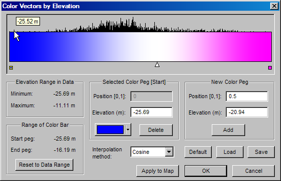
The large colored bar in this example represents a color range, which is calculated from the colors you assign to specific positions along the bar. The bar's left edge is at position 0.0 and the right edge is at position 1.0. You can assign colors to intermediate positions by creating one or more color pegs at appropriate points along the bar. The program will then calculate the colors for other positions using one of the interpolation methods described below. The cosine method illustrated here produces smooth color transitions between adjacent pegs. (The default method for depth coloring is HSL long, which can produce a good color range without intermediate pegs.) There is just one intermediate peg in this example, as indicated by the white triangular pointer -- white because that was the color assigned to it. You can create additional pegs in either of three ways:
| • | By double-clicking the bar, in which case the new peg's color and position depends on where you click. Although the peg's color is taken from the bar's original color at that position, which doesn't change, the colors on either side of the peg might change depending on the interpolation method. |
| • | By using controls in the New Color Peg section of the dialog, in which case you specify either the position or corresponding vector property (e.g., elevation). Again, the new peg's color is the original (unchanged) bar color at that position. |
| • | By dragging either of the two endpoint pegs (small squares) inward, toward the middle of the bar. When you start dragging a new triangular peg is created with the same color as the endpoint peg. You continue dragging to establish its position. As described below, this method is useful for reducing the range of data values that a color range represents. |
Whichever way a peg is created, it becomes the selected peg and the controls in the middle section of the dialog allow you to edit its properties. Normally you'll use the color selection button to change the color that was automatically assigned to a newly-created peg. Creating a peg, therefore, is usually a two-step process: fixing its position and editing its color.
You can select an existing peg via the keyboard (tab and arrow keys) or by left-clicking it with the mouse. The peg's properties can then be edited via the controls for the selected peg. Also, by left-dragging an intermediate peg, you can change its position without changing its color. In the above example, the left endpoint peg has been selected. This is indicated by the middle section's title, "Selected Color Peg [Start]", and by the fact that the leftmost small square is outlined.
Mapping Colors to Survey Vector Properties
When you use this dialog to define a color gradient, your goal will be to set it up so that the colors used to display survey vectors (or passage polygons) will reflect some vector property. The particular property is determined by the button you use to invoke the dialog and can be one of three types: elevation, date, or F-ratio. (Each of these types will be described in more detail below). In the dialog shown above, labels indicate that the property is elevation. Above the color bar is a histogram that shows the frequency of elevation values for vectors actually present in the data set. Here, the histogram covers elevations in the range -25.65 meters to -16.19 meters which have been linearly mapped to the gradient's position range (0.0 to 1.0). The yellow box with "-25.52 m" is what you see when you move the mouse cursor over a spike in the histogram representing an elevation of -25.52 meters. Every vector whose elevation falls within the color bar's range will correspond to a spike at least one pixel tall. Except for that condition, taller spikes correspond to larger proportions of vectors.
The mapping of gradient (color bar) range to elevation range is shown in the dialog section labeled Range of Color Bar. Displayed above this section, under Elevation Range in Data, is the range of elevations actually present in the survey database. These two ranges are automatically initialized to be the same when you first open this dialog to define a gradient for a compiled data set. Thereafter, the ranges might differ for two reasons. First, recompilations can cause the minimum and maximum values to no longer match the color bar range that's saved as part of the gradient's definition. Second, you can use this dialog to change the range of values represented by the color bar. The direct way of accomplishing this is to select one of the small squares representing an endpoint peg and edit its property value (elevation). In this example, the color bar's extent is smaller than the data extent.
Another way of reducing the bar's range that's easier than a direct edit, is to 1) add a new peg by left-clicking an endpoint box and dragging inward with the left button held down, 2) reselect the corresponding endpoint box and delete it. The peg you added by dragging disappears, but its property value and color are passed on to the "deleted" endpoint peg. The endpoint color doesn't change but the value it represents does. The bar's range is thereby reduced and the resolution of the histogram improves. When the map is drawn, vectors that have values outside the gradient's range will be given the color assigned to the appropriate endpoint peg. A variation on this method is to omit the deletion step (2) that improves the histogram' resolution. More likely, though, you'll be wanting to "zoom in" on the histogram. When choosing colors for a color-by-date gradient, for example, you might need to see separate spikes for two nearby dates.
The Reset to Data Range button will make the color bar limits correspond to the current minimum and maximum property values in the compiled item being reviewed. For all but the statistics gradient, all network components in the item, not just the selected one, will determine those limits. Besides applying to just the selected component, the statistics gradient is different in that this button also restores the default peg configuration, which is illustrated below.
The Apply to Map button updates any screen maps with the gradient you currently have defined -- but without exiting the dialog. This allows you to preview the gradient's effect as you make changes to it. Without this button you would need to commit to your changes by clicking OK, possibly replacing what may have been a more-acceptable gradient definition. If you Cancel the dialog, any changes you may have made to screen maps using this button are retained while the original gradient definition (and whether or not it is assigned to features) is unchanged. If necessary, you can use the Apply to Map button on the Segment page to refresh a map with the visibility attributes assigned to segment branches.
Saving and Restoring Gradients
When you assign any customized color gradient to a map feature, the current definitions for all three gradient types are saved in workfile <name>.NTAC, where <name> is the base name of the compiled project branch. Apart from this automatic feature, you can manually save and restore "snapshots" of the dialog's displayed gradient using the Save and Load buttons. That allows you to experiment with different color patterns while being able to quickly restore the gradient you normally use. A snapshot file, which stores both a gradient and the value range it represents, can have any name, but the extension is forced to be NTAE, NTAD, or NTAS, depending on the gradient type. As long as such files are kept in the project's work directory, they are considered part of the NTA file set that's optionally included in a backup archive.
The Default button replaces the displayed gradient and value range with what the program uses by default for a newly compiled data set (or one in which workfiles have been purged). If you never assign a customized gradient, no NTAC workfile is created.
Gradient Types
Here are some specifics regarding the three types of gradient coloring supported by this version of Walls:
| • | Color by Depth (Elevation) - The elevation of the vector's midpoint as determined from the compiled data. A units qualifier (ft or m) will indicate which distance unit is in effect during this review session. (See Review Units under Properties: General Page.) Note that the elevation range shown for the data set will not match exactly what you'll see in an Adjusted Totals report. Only the elevations of vector midpoints are relevant here. Also, all components of the reviewed data set, including all segment tree branches, "detached" or not, are considered when computing the data range and histogram. The default depth gradient for newly compiled project items is a blue-purple-red-yellow color range produced with the HSL long interpolation method (no intermediate pegs required). |
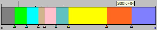
| • | Color by Date - The date assigned to a survey vector via the #Date directive. Vectors without assigned dates are lumped together and given the date 1000-01-01. Unless all vectors have unassigned dates, such vectors will not be used in the calculation of either the histogram or the minimum and maximum values. (When drawn they will be given the color assigned to the gradient's left endpoint.) You might want to use either the flat start or flat end interpolation method when coloring vectors by date. (The default for new compilations is a blue-to-red color range produced with the HSL long method.) Here is an example using the flat start method, the goal being simply to cover the relatively few different dates with a unique color: |
| • | Color by Stats (F-Ratio, or Consistency) - On the Geometry page of the review dialog, all traverses in loop systems are rated by their horizontal and vertical component F-ratios. The F-ratio is a positive number that's larger than one (and possibly quite large) when the traverse's presence in the data set is hurting overall consistency. When the F-ratio is less than one, consistency is being helped. The F-ratio used here to define a color gradient differs from those on the Geometry page in two respects. First, the one used here is a weighted average of the traverse's horizontal and vertical component F-ratios when those F-ratios are well-defined -- that is, when both component types haven't been completely constrained or floated. (The F-ratio of a vector in this context is the F-ratio of the traverse that contains it.) |
Second, we're using a global F-ratio, not one specific to the independent loop system containing the traverse. Whereas the system-specific F-ratios shown on the Geometry Page can be misleadingly large when a system has few loops, the global F-ratio measures a vector's consistency with respect to all systems in the connected component. The component possibly contains many loop systems. The histograms of the other gradient types are even more inclusive since they represent all vectors in the compiled data set, not just the selected component.
In statistics gradients, three special values are reserved to represent vectors that don't have F-ratios. Vectors for which both component types (horizontal and vertical) are constrained are assigned value -1.0. Vectors for which both component types are floated are assigned value -2.0. Vectors not contained in any loop are assigned value -3.0. The statistics gradient assigned by default (and which is restored by the Reset to Data Range button) looks like this:
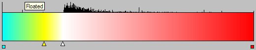
With this gradient selected, non-loop vectors will be colored light blue, floated vectors will be colored green, and constrained vectors will be colored yellow. Normal loop vectors, with F-ratios 0.0 or greater, will have colors ranging from white to red. Here we're using linear, not cosine, interpolation to produce a faster transition to red (see below). Note that the leftmost spike in the histogram, which represents non-loop vectors, is no taller than the tallest of the remaining spikes. The program enforces this to ensure that a large proportion of non-loop vectors doesn't flatten too severely the remaining part of the histogram.
Interpolation Method
The program uses one of several interpolation methods to calculate color as a function of position along the bar. To change the appearance of the bar without affecting the current peg colors, you can specify one of the following algorithms:
| • | Linear - Each of the three RGB (Red, Green , Blue) color components is obtained as a weighted average of the corresponding color components of the two adjacent pegs. |
| • | Cosine - Similar to linear, except that the weighting is based on the cosine function, causing somewhat smoother transitions across pegs. |
| • | Flat start - Moving left to right, the color abruptly changes from that of the previous peg to that of an encountered peg. The bar has N+1 distinct colors, where N is the number of intermediate pegs. This method is useful for date coloring when there are only a few dates, or date ranges, to distinguish between. |
| • | Flat end - Similar to flat start. In the above description change "left to right" to "right to left." |
| • | Flat Middle - The color at a position is the unweighted average of the two adjacent peg colors. |
| • | Reverse - Linear interpolation calculated in reverse. Moving left to right, instead of starting with the current peg's color and transitioning smoothly to the next, it starts at the next color and transitions to the current peg's color. |
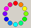
| • | HSL CW, HSL CCW, HSL Short, and HSL Long - These four methods interpolate between adjacent pegs by treating their colors as points on the HSL (Hue, Saturation, and Luminance) color wheel. |
|
Since the wheel is circular, there are two possible routes to take when transitioning from one peg's color to that of an adjacent peg. The HSL CW and HSL CCW methods take the clockwise and counterclockwise routes respectively. HSL short and HSL long take the shortest and longest routes respectively. With the HSL methods you don't need intermediate pegs to produce rainbow-like effects. The default depth and date gradients are produced this way using HSL long with suitable colors chosen for the endpoint pegs. |
In designing the gradient dialog, I borrowed from the work of programmer Joel Holdsworth. (See Acknowledgements.)
For more information on selecting gradient coloring for map features, see Color selection Palettes.